Lesson 7.2 The Central Limit Theorem for Means or Averages

Notation and Formulas 

X is a random variable with a distribution that may be known or unknown. Using a subscript that matches the random variable, suppose

• μ_X = the mean of X.
• σ_X = the standard deviation of X.

If you draw random samples of size n, then as n increases, the random variable

of the sample averages tends to be normally distributed as follows:

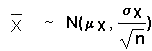
Notice that the mean of the sample averages is the same as the mean of the original distribution, but the standard deviation of the sample averages is the standard deviation of the original distribution divided by the square root of n.

 

Back to Top

Law of Large Numbers

The Law of Large Numbers says that if you take larger and larger samples from any population, then the sample mean gets closer to the population mean. The Central Limit Theorem (CLT) says that as the sample size n gets larger, the sample means follow a normal distribution. As n gets larger, the standard deviation for the averages gets smaller. As the standard deviation for the averages gets smaller, the sample means get closer to the population mean.  

CLT Problems for Averages Using TI-83 or TI-84 calculators

Example: The length of time, in hours, it takes an "over 40" group of athletes to play an indoor soccer match has an unknown distribution. The mean is 1 hour and the standard deviation is 0.5 hours. Suppose, 25 of these soccer matches are randomly chosen.

Let X = the length of time, in hours, it takes to play one of these soccer matches. Then,

and follows a normal distribution:

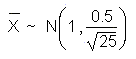
where μ_X = 1 and σ_X = 0.5.

 

Below are some typical problems. The answers have been calculated using technology (TI-83 calculator).

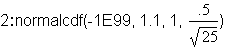
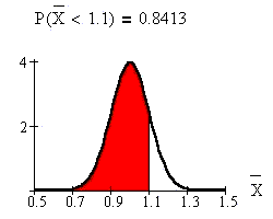
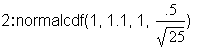
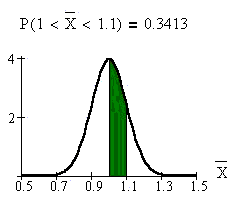
What is the probability that the average length of time of 25 soccer matches is less than 1.1 hours?   The probability that the average length of 25 soccer matches is less than 1.1 hours is 0.8413. This calculation was done using TI-83 or TI-84 calculator function 2nd DISTR. What is the probability that the average length of time of 25 soccer matches is between 1 and 1.1 hours? The probability that the average length of time of 25 soccer matches is between 1 and 1.1 hours is 0.3413. This calculation was done using TI-83 or TI-84 calculator function 2nd DISTR. 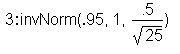Find the 95th percentile for the average length of time of 25 soccer matches. Let k = the 95th percentile (95%ile). 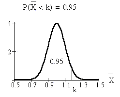k = 1.17 (to 2 decimal places). The 95th percentile is 1.17 hours. This means that 95% of the average lengths of soccer matches are less than 1.17 hours. This calculation was done using TI-83 or TI-84 calculator function 2nd DISTR. The IQR (interquartile range) for the average length of a soccer match is from ____ to ____. IQR = ____ The IQR is the spread of the middle 50% of all average lengths of soccer matches. IQR = Q3 - Q1. 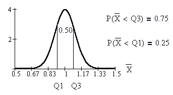Q3 = the 75th percentile and Q1 = the 25th percentile     Q3 = 1.07 and Q1 = 0.93 (to 2 decimal places). These calculations were done using TI-83 or TI-84 calculator function 2nd DISTR. 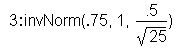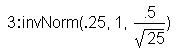The IQR goes from 0.93 to 1.07 hours. IQR = 1.07 - 0.93 = 0.14 hours.

Examples

1) The following problem is concerned with the average percent of calories from fat that a person from the United States consumes. Close the window when you are finished viewing the example. You will return here.

2) The next example is concerned with the average stress score of students. The stress scores follow a uniform distribution but, by the CLT, the average stress scores follow a normal distribution. Close the window when you are finished viewing the example. You will return here.

Back to Top

Think About It

The length of time to brush one's teeth is generally thought to be exponentially distributed with a mean of 0.75 minutes.

• Find the probability that the average time it takes 50 people to brush their teeth is more than 0.8 minutes.
• Find the 95th percentile for the average time it takes 50 people to brush their teeth.

For the probability problem, use your calculator and the normal CDF function (normal CDF on the TI-83). The mean of the averages is equal to the original mean. The standard deviation of the averages is the original standard deviation (it is 0.75, the same as the mean) divided by the square root of the sample size.

The range of average times goes from 0.8 to 1EE99. Answer is 0.3187. For the percentile problem, use the inverse norm function (invNorm on the TI-83). The area to the left is .95. Answer is 0.92.

This is the last required section of this lesson. Please continue to the optional section of this lesson. When you have completed the assignment and the quiz for Lesson 7, you are ready to begin Lesson 8 - Confidence Intervals.

Please continue to the next section of this lesson.

Back to Top

Up » 7.1 Central Limit Theorem » 7.2 Central Limit Theorem for Averages » 7.3 Central Limit Theorem for Sums